MultiScale Microscopy Detailed
| Title | MultiScale Microscopy Detailed |
|---|---|
| Summary | Master Thesis Project |
| Keywords | |
| TimeFrame | |
| References | |
| Prerequisites | |
| Author | Amir Etbaeitabari, Mekuria Eyayu |
| Supervisor | Stefan Karlsson, Josef Bigun |
| Level | Master |
| Status | Internal Draft |
Contents
[hide]Summary
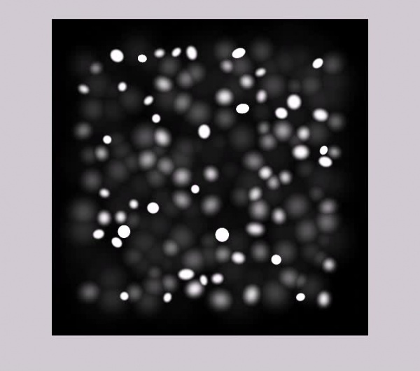
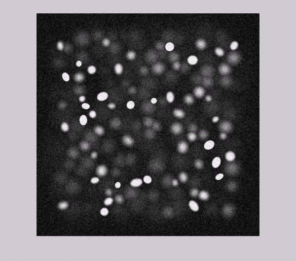
Counting white blood cells in microscopic images is a tool for physicians to diagnose the human body health condition. The aim of this project has been twofold. Firstly, we made an application for synthesizing data with known ground truth objects. These objects are elliptical in appearance of five different classes within in a volume by considering the depth of focus (DOF) 15 photos are taken (captured) from the volume at different depth (see examples below). Secondly, we provided an algorithm that exploits the multiscale nature of the problem in order to improve recognition. The variation of gray value for each pixel in different depth is used as feature source for classifier. The classifier divides the pixels in three different groups, background pixels, pixels in single cells and pixels in overlapping parts. For counting the total number of cells, centroids of overlapping areas are used for bisecting the overlapping ones. The final result contains different models varying noise density and resolution, which contains accuracy of overlapping positions and area of overlapping found correctly in the image. In non-noisy environment the performance for accuracy of overlapping positions is x1 % and for area of overlapping places is y1 % for density of 150 cells and is x2 % and for area of overlapping places is y2 % for density of 200 cells.
Introduction
Counting white blood cells from microscopic images is a tool for physicians to diagnose human body health condition. Providing a large clinical data set is necessary for calculating performance measurements of different segmentation algorithms. In spite of hard accessing to datasets, experts are needed to use visual analysis to obtain the “Golden Ground Truth’’. In addition, there are negative factors like noise, poor image quality and variant illumination which make it harder to extract the ground truth.
In our project, we have introduced an algorithm for making different models of volumes containing cells with some flexible parameters .The requested numbers of elliptical cells of different classes are generated randomly inside a defined volume. The analyzers could have access to the ground truth for evaluation of the performance. Furthermore, the effect of variation in factors like noise, resolution and illumination variance can be studied independently or in combination in our models. The synthesizing algorithm provides an opportunity to analyzers to experience and consider different conditions and environment properties such as different cell density, noise density and resolution by varying different factors in the algorithm for generating different cell models. Requested numbers of photos by user are captured by a virtual fixed camera by changing its focal length while focusing at different equidistant depths in a volume. Depth of focus effect for cells in different depths is considered.
Identifying overlapping areas (positions) and counting the total number of cells in different environments is our main concerns in this project. For an environment with predefined constant brightness, a method using the gray value average of all depths is applied for finding the overlap places due to its simplicity, less computational time and efficient results. The average of gray values from the sequence of photos besides defining a threshold is used for this approach. Furthermore, different features such as the magnitude of discrete Fourier transform and 1D derivation of the sequence of each pixel gray values in the depths are extracted ´. After preprocessing the data, it is given as input to linear and neural network classifiers to make a robust algorithm for classification of each pixel in three different groups, background pixels, pixels in single cells and pixels in overlapping parts, by considering different noise densities and photos with different resolutions. The results are compared with some pervious works.
Background
Developing a robust algorithm for Identifying and separating overlapping particles in a microscopic images is one of the main concerns and research work for computer scientists. The current overlap separating approaches are based on prior particle shape and gray value intensity. Like watershed method [10,11], and mathematical morphology method [3,8,9] faces an over segmentation problems and expensive in computational time. [xxx]
According to [Gloria Diaz,Fabio Gonzalez and Eduardo Romer] they proposed a static template matching for a specific cell class knowing their prior knowledge of the cell shape and size. They construct a single cell template model to identify the overlapping particles. However, their approach could not be used for many cell classes which contain different sizes of single cells as well as complex overlapping cells. The approach for separating touching and overlapping objects by [Jose M.Korath, Ali Abas, Jose A.Romagnoli] uses geometrical features and variation of intensity in the places of touching and overlapping places. For noisy and poor resolution images the gray value feature will introduce an error in identifying overlapping objects. Besides, we got a 70% performance for identifying the overlapping places using their methods. Finally, for the total cell counting and segmentation we have used the classical watershed algorithm as a comparison with our approach. Since, we are using 15 layers of multi scale microscopic images as input, where each slice contains some information of the entire particle density in a volume, for a fairly segmentation and cell counting process comparison ,we even gave the ground truth as an input to watershed instead of the slice images. However, it results in an over segmentation outcome.
Method
Synthesizing a Multi layered Microscopic Images
In our model we have considered a 3D volume which can contain different cells inside, with their specific x, y and z coordinates. As we know in real world, most of the microscopic cells have a circular or ellipsoid like shapes. Hence, we have used a general ellipse equation in order to model the real cells.
An ellipse is a curve described implicitly by an equation of the second degree Ax2+ Bxy + Cy2 + Dx + Ey + F = 0 when the constraint B2 - 4AC is less than zero.
In a simplified approach we can represent an ellipse with centres at (<math>x_{c},y_{c})</math> could be expressed using a general equation as:
- <math>{A}{(x - X_c)^2}+ {B}{(x - X_c)}{(y - Y_c)^2}+{C}{(y - Y_c)^2}=1</math>
Furthermore, for a cell which has a defined Area A and circularity β, we can represent the general ellipse equation using matrix notation by applying rotation and translation as follows:
- <math>{r^T}R_{\theta}^{T}\begin{pmatrix}{{\beta}^{2}}\frac{\pi}{A} &\frac{B}{2} \\ \frac{B}{2} & {{\beta}^{-2}}\frac{\pi}{A}\end{pmatrix} R_{\theta}{r} = 1</math>
where <math> r= \begin{pmatrix}x - X_{c} \\ y - Y_{c}\end{pmatrix}</math> and <math> R_{\theta}</math> is the rotational matrix for angle <math>{\theta}</math> (the rotational of the ellipse dominant direction, which is randomly chosen for each cell in our model). And the coefficients A, B and C of the ellipse equation should be calculated from the matrix notation expression.
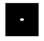
For illustration purpose we have produced cell samples with circularity <math>{\beta}=0.8</math> and <math>{\beta}=1</math> respectively as shown below.
By considering the Depth Of Field, we generated multi layered microscopic images from our synthesized data . We have used Gaussian filters to blur the image of each cell with respect to the distance of its depth in the volume from the the focal point of the camera in that corresponding image.
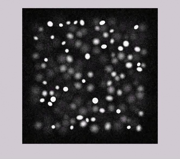
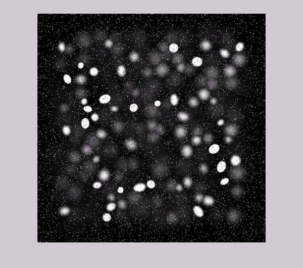
Sample of Synthesized Microscopic Images :
Current thumbnail generation does not work for the encoding on this page. Press play on the videos below to get a better view of what the data looks like. Encoding is .OGG and distorts the appeareance slightly (lossy compression).
Pure Data:
With Additive Gaussian noise:
With Salt and Pepper noise:
Methods for classification
Data Preprocessing
Standardization is applied on the data set to deal with features with different scales. It transforms each feature in data set to have zero mean and unit variance.
Principal Component Analysis method (PCA) is then applied on the standardized data. It makes an orthogonal transformation to the data set into new linearly uncorrelated features space.
Feature Selection is done by Backward Feature Elimination and checking the generalization error to guarantee that all used features are beneficial.
Classifiers
Linear classifier and Neural Networks are used to classify all pixels into 3 different classes, background pixels,pixels captured by single cells and pixels captured by areas of overlapping in 2D output image.
Linear classifier is used due to its simplicity, speed of classification and as a measurement for comparison to more complex models, here Neural Networks.
Neural Network with one hidden layer is used for classification as a nonlinear classifier. The complexity of the Neural Network, number of hidden nodes,is decided by the least generalization error while changing the node numbers.
Watershed
The output of the classification part is used as the input for counting cells part.For comparing the result of counting cell part of the project with previous works, Watershed algorithm is chosen as one. Watershed uses binary images as its input. As it is presented in the videos, none of the 15 photos contain all information about the volume. Therefore, instead of using a binary image from one of the photos, the binary image of the ground truth is used as the input for watershed.In spite of giving this privilege to Watershed Algorithm here, it will be shown that the counting result of watershed algorithm suffers from over segmentation.
Our method for counting cells and bisecting overlapping cells
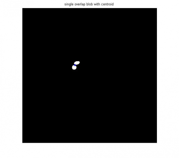
We have used the neural network output, overlapping areas from a volume filled with defined density of cells, to generate a vector of overlapping area centroids in order to use them for bisecting overlapping cells.
By marking all the centroid points of overlapping areas of the overlapping cells, we identify the nearest background pixel around the edge of overlapping cell by using Euclidian distance. The line crossing this pixel and the corresponding centroid point, by some modifications, is considered as the bisecting line for those overlapping cells.
As, we mentioned in sec xxy our model considers a noisy environment and images with different resolutions. It is likely to miss a few overlapping areas which leads to assign those overlapping cells as single cells.
To overcome such problems, we have also used some geometrical properties as additional features for the final step of cells counting. Experimentally, we have found that circularity, area and extent features of an object are very important and can be easily used to distinguish single cells from those overlapping cells which are left not bisected from the previous phase.
Finally, by fusing the result from the bisecting cell method and the geometric features extraction method, we are able to count the total number of cells with in a volume filled with cells.
Pictorial Illustration for of our Algorithm during bisecting overlaps and counting
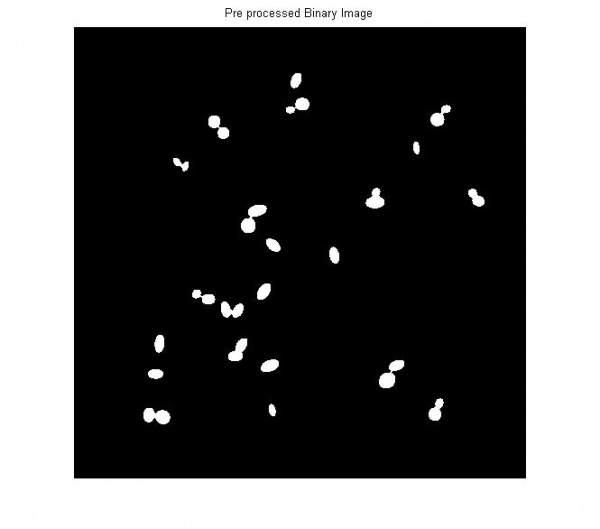
We have used binary image output from classifier which is an input to our algorithm and watershed for counting the total number of particles in a given volume.
Figure: Input Binary Image from classifier containing 150 cells
Figure: Pre Processed Input Binary Image
Figure: drawing a bisecting line in overlap cell
Figure: drawing a bisecting line in overlap cell in high resolution image
Figure: overlapping cell afeter bisection
Figure: watershed segementation result with Low resolution
Comparison between watershed algorithm and Our approch
To notice the oversegementation result of watershed with respect to our method we have comapared same two overlapping cells as follows:
Figure: watershed segementation for overlap cell
Figure: segementation using our method for overlap cell
Analysis Method or Test (Experiment) Setup:
As we mentioned in section xx1, we have tried to compare our approach based on a classifier which uses the features (1D derivation, FFT and the Moments) of the 15 scaled photos as an input with the [Jose M.Korath, Ali Abas, Jose A.Romagnoli] which uses variation of intensity.
Experiment 1
For Experiment1 we used an averaged gray value image, obtained from 15 scaled photos, as an input to analyse the system. External factors like noise and resolution are considered.
Experiment 2
Similarly for Experiment2 we combined different features (1D derivative, FT and Moment) of the 15 scaled photos as an input to a classifier (Neural Networks and Linear models) External factors like noise and resolution are considered.
Experiment 3
Here we have compared our approch with watershed algorithm for counting the total number of particles inside a volume and the performance result is shown using bar graph.
Results
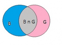
The graphs below illustrate the performance of finding overlapping particles in a noisy environment and different resolution images. We have used a Venn diagram for illustrating the accuracy in finding overlapping positions, where B is for our model output, G is for ground truth image and B n G is their intersection. For measuring the relative overlapping particles we have used the Dice coefficient[Dice LR. Measures of the amount of ecologic association between species ecology.J Ecology. 1945;26:297–302.] which is mostly used for measuring spatial overlap for binary images. The Dice coefficient D is given by <math> D=\frac{2|B n G|}{|B|+|G|}\times 100</math> and the values for the coefficients varies from 0 (non overlap) and 1 (perfectly overlapped).
Result 1
Figure 1:Performance versus noise density using State of art
Figure 2:Performance versus Resolution using State of art
Result 2
Figure 3:Performance versus noise density using Linear network
Figure 4:Performance versus noise density using Neural network
Figure 5:Performance versus Resolution using Linear network
Figure 6:Performance versus Resolution using Neural network
Result 3
Figure 8:Performance versus number of cells
Conclusion
As we described in sec xxx we have compared the output results between state of art and our method in noisy environment and also independently, in images with different resolutions.
The performance result using the state of art is around 70%. Similarly, by using our approach we have improved to 93% in noise free environment, with highest resolution images (i.e. 1000x1000 pixels) by the neural network classifier.
By taking 70 different models which contains 1106 overlapping places of ground truth image (reference image) and the missing overlaps from classifier output is 18 with respect to ground truth image. Hence, the performance of the missed overlaps is around 98.4%, which is better than the performance measure using disc.
In our case, 8 features are extracted for each observation. According to Hermmetian symmetry in Discrete Fourier Transform coefficients the magnitude of the first eight ones are chosen to describe each data element for classification using linear models and neural network while [Jose M.Korath, Ali Abas, Jose A.Romagnoli] use one of the 8 features which is the dc part , average gray value intesinisy.
Similarly, we have compared the performance of total cell counting between water shed approach and our method in different cell density models (i.e. 100,150, 200,250 and 300).
The cell counting performance, in noise free and high resolution images, using water shed in different cell density models varies from 20% to 25 %, while our method performance varies from 95% to 99%.
The performance of counting cells for water shed is calculated in a situation that water shed algorithm was fed with the ground truth 2D image, to compare the water shed result with ours in a fair way.
Even by accessing to Golden Ground Truth, watershed suffers too much from over segmentation that causes a visible difference between watershed output and our method output in cell counting even when we are using our classifier output (not the ground truth).
Future work
In the synthesizing part, a complete 3D model can be designed which can be viewed from different angles, and also a pattern can be added to cells structures as a future work.
Meanwhile, for the performance measure of overlapping places it can be used another accuracy measurement like Gaussian function and tent function for expressing the performance accuracy in a more fuzzy way.
